R has four standard functions for specific ways that numbers can be distributed. In general, the names of the functions begin with either r, d, p, or q and end with an abbreviation for a kind of distribution. For example, runif is the r function for uniformly distributed numbers while rnorm is the r function for normally distributed numbers.
The r version of these functions is the easiest to understand. It returns a specified quantity of random numbers with the desired distribution (r = random).
   # unif defaults to min=0, max=1
> runif(3)
[1] 0.427 0.945 0.520

   # norm defaults to mean=0, sd=1
> rnorm(3)
[1]  0.710 -0.953  0.609
The r versions of the distribution functions allow you to create sets of numbers with known properties, such as means and standard deviations. You can then test statistical formulas against these to see how often they provide the correct answer with various sample sizes and other numerical characteristics. This is a thoroughly modern method for learning statistics.
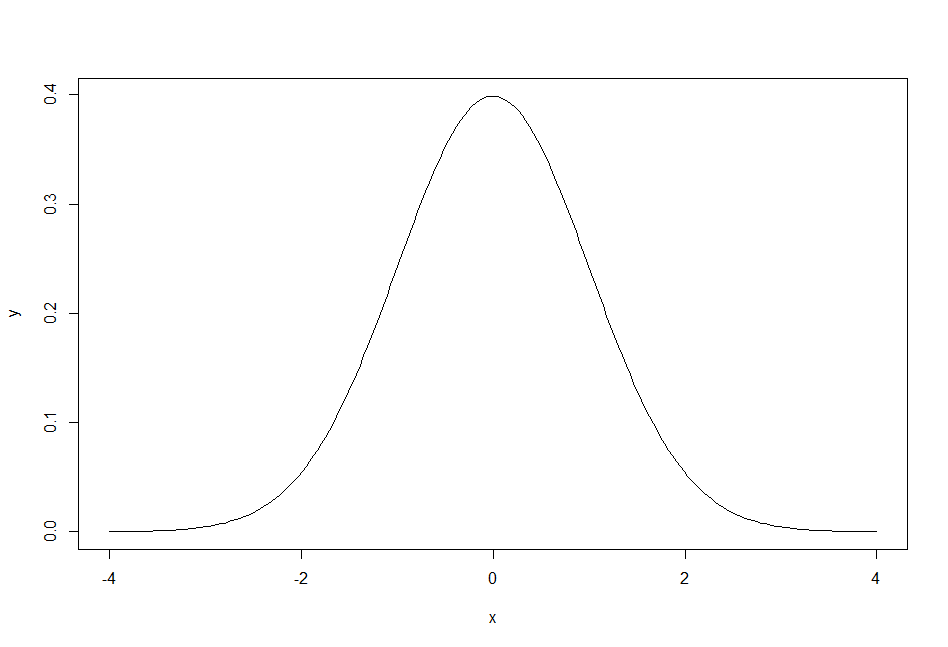
To understand the d version of the distribution functions, think of the bell curve graph that’s associated with the normal distribution. On this graph, the x-axis specifies a range of numbers from smallest to largest . The y-axis shows the density of the distribution at each of those numbers (d = density).
In the bell curve for a normal distribution, the highest point will be at the mean (that is, when numbers are distributed normally, there are relatively more numbers near the mean). The lowest points will be at the tails (in a normal distribution, there are relatively few numbers near the minimum and maximum numbers). To actually draw a bell curve for a theoretical distribution, you’d need to know the y-value to use for the numbers on the x-axis. The d versions of the distribution functions tell you the y-axis density value for the x-axis numbers, given the specified distribution.
# Unif density is the same everywhere
> dunif(c(.05, .5, .95))
[1] 1 1 1

   # Norm density is highest near the mean
> dnorm(c(0, 1, 1.96))
[1] 0.39894228 0.24197072 0.05844094

   # How to plot a normal curve
> x = seq(-4, 4, length.out = 200)
> y = dnorm(x)   # get normal density at each x
> plot(x,y, type="l")
The p version of the distribution functions gives the area under a curve of the distribution that is to the left of the number you specify, where the total area under the curve is 1. You can also think of this as the probability that there are numbers in the distribution that are equal to or lower than the numbers (typically statistical test scores) you specify, or as the proportion of numbers that are equal to or lower than the distribution quantiles you specify, or as the percentile of those numbers in the distribution you specify (p = proportion or probability or percentile).
   # unif defaults to min=0, max=1
> punif(c(.05, .5, .95))
[1] 0.05 0.50 0.95

   # norm defaults to mean=0, sd=1
> pnorm(c(0, 1.64, 1.96))
[1] 0.500 0.949 0.975
Finally, the q version of the distribution functions allows you to specify numbers between 0 and 1 that represent one or more probabilities, proportions, or percentiles. The function returns the quantiles (or, typically, statistical test scores) that are associated with those probabilities or proportions or percentiles in the given distribution (q = quantile).
   # unif defaults to min=0, max=1
> qunif(c(.05, .5, .95))
[1] 0.05 0.50 0.95

   # norm defaults to mean=0, sd=1
> qnorm(c(.5, .95, .975))
[1] 0.000 1.645 1.959
Note that the p and q versions of the distribution functions are opposites in that each returns the values that are specified in the alternate function. The p version always returns numbers between 0 and 1 and the q version always requires you to specify numbers between 0 and 1. Which function you use depends on what you already know and what you need to know.
At the back of most statistics books you’ll find a series of tables; the p and q versions of the distribution functions are the R equivalent of these tables. Use the p version if you have a table’s marginal value and want to get the probability associated with that value. Or use the q version if you have a probability and you want the table’s marginal value.
For example, the body of a Normal Probability Table shows Z-Scores in the table margins and the probability of those Z-Scores in the body of the table. You can think of the p version of the distribution functions as requiring a score and returning a probability and the q version as requiring a probability and returning a score. Thus the p and q versions of the distribution functions duplicate what those tables in the back of your statistics textbook do.
   # Z-Score to probability:
> pnorm(1.01)
[1] 0.8438

   # Probability to Z-Score
> qnorm(.8438)
[1] 1.0101
In the following posts, I’m going to use these functions to demonstrate how the formulas you learn in statistics classes work.